Quantum gis

General QGIS info

Features

The major features of QGIS include:

Direct viewing and exploration of spatial data
- Advanced symbology (edit rendering styles)
- QGIS Browser as a simple and fast data viewer
Support for numerous vector, raster, and database formats
- ESRI shapefiles, GeoJSON, KML/KMZ, and GPX
- PostGIS, PBF, SpatiaLite, MSSQL spatial, WMS
Create, edit and export spatial data
- Work with nodes, lines and polygons
- Convert between different coordinate systems (re-projection)
- Down/upload directly to a GPS unit
Perform spatial analysis
- Find polygon centroids and basic statistics
- Distance matrix and line intersections
Publish your map on the internet
An extensible plug-in architecture

Other useful pages to bookmark:

Coordinate Reference System

Earth is a three-dimensional body, roughly spherical in shape, yet the vast majority of maps are flat (2-dimesional). A Coordinate Reference System (CRS) defines a method of projecting all or part of the Earth onto a 2D surface. QGIS has support for approximately 2,700 known CRS. Some, such as WGS-84 are global projections, whereas others represent only specific regions.

Setting the CRS

When working with geo-spatial data it is essential that you are using the correct CRS. If you are lucky the projection will be specified as part of the vector file (for example, ESRI Shapefiles often include projection data in the .prj file), however you will often have to manually select the correct CRS.

To specify the CRS of a vector layer, select the layer and choice Layer->Set CRS of Layer(s)…. Each layer can have a different CRS. If this is the case, you will need to convert them to the same CRS in order for them all to display correctly. The easiest way to do this is to use ‘on the fly’ CRS transformation:

Settings->Project Properties (or click on the globe symbol in the lower right corner).
Select the Coordinate Reference System (CRS) tab.
Check the Enable ‘on the fly’ CRS transformation checkbox.
Pick a suitable project CRS to work with (e.g. WGS-84).

Using QGIS to convert between CRS

QGIS can be used to convert between CRS. Open the input layer making sure to select the correct CRS as described above. Use Layer->Save As… to export the layer with a different CRS (you may choice between the «Project» CRS or select a CRS from QGIS’s extensive list).

Using QGIS to filter data from government sources and convert it to KML

In Sweden multiple government agencies give out data in large shapefiles. These files do not load nicely in JOSM because of their size and/or JOSMs premature shp support.

To filter out part of a shp file in QGIS you can do this:

open the shp file in QGIS
enable editing
select a number of nodes and delete them
rightclick on the layer and choose «Export..»
select KML (this is better supported in JOSM)
click save and open up the result in JOSM

[править] Разграфки

Gimp

Номенклатурные сетки-разграфки карт — полигональные векторные слои, представляющие официальную номенклатуру, где каждый полигон описывает границы одного стандартного листа.
Масштабы: 1:1 000 000, 1:500 000, 1:200 000, 1:100 000, 1:50 000, 1:25 000

Сетка-разграфка 1х1 и 5х5 градусов для данных SRTM .

Разграфка WRS-1 и WRS-2 для данных Landsat — описание системы разграфки данных и сама схема для загрузки.

Схема зон UTM/GK — позволяет определить, в какой зоне находятся ваши объекты, можно использовать разграфку зон Гаусса-Крюгера, Universal Transverse Mercator. Есть возможность скачать разграфку в формате: ESRI Shape, Mapinfo TAB, KMZ.

Схема фрагментов для продуктов MODIS 2G, 3, и 4 — описание системы «нарезки» данных и сама схема для загрузки.

Стандартная номенклатурная разграфка топографических карт

Procedure¶

Rider plugins
Locate the downloaded file in the Browser panel. Expand it and drag the file to the canvas.

You will see a new line layer called added to the Layers panel. This layer represents each road in Washington DC. Select the Identify tool in the Attributes Toolbar. Click on any road segment to see what attributes are attached to it. There are standard attributes like Route-name, Road-type etc. there is an attribute called . This is an import attribute for routing as it specifies whether the segment is two-way or one-way. It contains 4 different values. (Both Directions) for two-way streets. (Out Bound) for one-way streets where the traffic is allowed in the direction of the line (start-point to end-point) and (In Bound) for one-way streets where the traffic flows in the opposite direction of the line. There is also value where we will assume two-way traffic. We will now use the information in that attribute to display an arrow on one-way streets.

Click the Open the layer Styling Panel button in the Layers panel. Select the renderer from the drop-down menu.

We will create a new style with a filter for only the one-way roads. Click the Add rule + button.

In the Edit rule dialog, click the Expression button.

In the Expression string builder dialog, expand the Fields and Values section in the middle-panel. Select the attribute and click All Unique in the right-hand panel. The 4 values that we discussed earlier will appear. Having these values here as a reference helps when building the expression. Also, you can double-click on any value to add them to the expression.

The goal is to create an expression that selects all one-way streets. Enter the following expression and click OK.

Next, change the Symbol layer type to .

Select under Marker placement.

Click on the symbol. Scroll down and pick the marker. You will see that the arrow-like symbol now appears on the one-way streets. But all of them are pointing in a single direction, whereas we know that our filter contains roads in multiple directions. We can further refine the symbols with a data-defined override for the Rotation value.

Click the Data defined override button next to Rotation.

We can put a conditional expression that returns different rotation values depending on the one-way direction. A 180° degree rotation for the road with opposite direction will make the direction perfect, In this, we will make the Roads with attribute rotate 180° hence all roads will have the correct traffic flow direction. Enter the following expression and click OK.

Now you will see the arrow-heads aligned to the correct road direction. To keep the style uncluttered, we are choosing to display arrows only on one-way streets. Unlabeled streets are assumed to be two-way. Now that we have the network styled correctly, we can do some analysis. Go to Processing ‣ Toolbox.

Search for and locate the Network analysis ‣ Shortest path (point to point) algorithm. Double-click to launch it.

In the Shortest Path (Point to Point) dialog, select as the Vector layer representing network. Keep the Path type to calculate as . Next, we need to pick a start and endpoint. You can click the … button and click on any point on the network in the canvas. If you want to replicate the results in this tutorial, you can enter as the Start point and as the End point. Expand the Advanced parameter section. Choose as the Direction field. You must be familiar with the one-way direction values for the forward and backward traffic flow. Enter as the Value for the forward direction and as the Value for the backward direction. Keep other options to their default values and click Run.

The algorithm will use the geometry of the layer and provided parameters to build a network graph. This graph is then used to find the shortest path between the start and endpoints. Once the algorithm finishes, you will see a new layer added to the Layers panel that shows the shortest path between start and endpoints.

You will see that there are many possible paths between start and endpoints. But given the constraints of the network — such as one-ways, the result is the shortest possible path. It is always a good idea to validate your analysis and assumptions. One easy way to validate it is to use a third-party mapping service to see if their results match with the ones we derived. Here is the shortest path suggested by Google Maps between the same start and endpoints. As you can see the recommended shortest route matches exactly with our results — validating our analysis.

Выражения¶

Mcneel rhinoceros на русском 6.28.20199.17141

There is now a string format parameter available for the function in QGIS expressions. Users now have various options that they can use to stipulate the format of the returned UUID value, including the following options:

: {0bd2f60f-f157-4a6d-96af-d4ba4cb366a1}
: 0bd2f60f-f157-4a6d-96af-d4ba4cb366a1
: 0bd2f60ff1574a6d96afd4ba4cb366a1

This feature was developed by signedav

QGIS expressions now support a layer_crs variable which will return the AuthID for a particular layer’s coordinate reference system. This allows expressions to identify the layer CRS dynamically and perform transformations without needing to manually specify the CRS.

Разработчик — Alex

QGIS expressions now include aggregate functions for arrays, which allow the easy retrieval of specific values from an array that may be used in QGIS elements such as symbologies. The following functions have been introduced:

array_min
array_max
array_majority
array_sum
array_mean
array_median

Разработчик — uclaros

The function array_get now supports the use of negative index positions.

Разработчик — Alex

Get involved with the community

New features and enhancements

If you wish to contribute patches you can:

fork the project
make your changes
commit to your repository
and then create a pull request.

The development team can then review your contribution and commit it upstream as appropriate.

If you commit a new feature, add to your commit message AND give a clear description of the new feature. The label will be added by maintainers and will automatically create an issue on the QGIS-Documentation repo, where you or others should write documentation about it.

For large-scale changes, you can open a QEP (QGIS Enhancement Proposal). QEPs are used in the process of creating and discussing new enhancements or policy for QGIS.

Translations

Please help translate QGIS to your language. At this moment about forty languages are already available in the Desktop user interface and about eighty languages are available in transifex ready to be translated.

Data Management¶

A new “Show CRS accuracy warnings for layers in project legend” is provided which, when checked, will display a new warning icon identifying any layers with a CRS which is identified as having accuracy issues.

Examples of low-accuracy layers might include those with a dynamic CRS with no coordinate epoch available, or a CRS based on a datum ensemble with accuracy that is found to exceed the user-set limit.

This option is disabled by default, and designed for use in engineering, BIM, and other industries where inaccuracies of meter/submeter level are very dangerous.

This feature was developed by Nyall Dawson

Basic support for the coordinate epoch of dynamic (not plate fixed) CRS has been added in line with relevant updates to GDAL.

QGIS has added support for respecting the source or destination coordinate epoch when transforming to or from a dynamic CRS.

If a dynamic CRS to dynamic CRS transformation at different epochs is attempted, which is not currently supported by PROJ, a user-facing warning message will be shown advising them that the results may be misleading and should not be used for high accuracy work.

This feature was developed by Nyall Dawson

Various improvements have been made to the handling and representation of projection information in QGIS, including:

The addition of an API to retrieve PROJ operation details for CRSes
The ability to show extended information about a layer’s CRS in the layer properties info tab, including accuracy warnings
The addition of a variable, for retrieving a friendly name of a map’s projection (e.g. “Albers Equal Area”)

This feature was developed by Nyall Dawson

QGIS now shows a warning in the projection selection widget when a CRS based on a datum ensemble is selected, warning the user that there’s an inherent lack of accuracy in the selected CRS.

This feature was developed by Nyall Dawson

A “persist layer metadata” checkbox has been added to the export vector file dialog. When checked, any layer metadata present in the source layer will be copied and stored in the destination file.

This functionality is enabled by default and ensures that metadata is properly transferred over to newly created items, which is especially effective when utilizing the GPKG format.

This feature was developed by Nyall Dawson

QGIS now supports “layer notes”, which can be created via the “Add Layer Notes” action in the layer context menu.

These notes are saved per layer, per project. They can be used as a place to store important messages for project users, such as to-do lists, processing or management instructions, or any other arbitrary text-based metadata.

A notepad indicator icon in the layers panel identifies layers that have notes attached. Clicking the notes indicator icon will open the note for editing.

This feature was discussed in QEP-206

These notes may be copied and pasted using the traditional copy/ paste methodology for transferring styles between layers in QGIS.

Layer notes are also supported by and stored within QML (QGIS Style) and QLR (QGIS Layer Definition) files.

This feature was funded by Alta Ehf

This feature was developed by Nyall Dawson

QGIS will now automatically load and convert ESRI metadata stored using a .shp.xml sidecar file. Where shapefile data is loaded and these metadata files are present they will be loaded automatically, with available layer metadata populated accordingly.

This feature was developed by Nyall Dawson

When loading data from a .gdb file, QGIS will automatically attempt to translate as much as possible of the original ESRI metadata across to the QGIS metadata, so that it’s immediately available for use.

This feature was funded by North Road / SLYR

This feature was developed by Nyall Dawson

For formats that support the embedded definition of field domains (currently GPKG and GDB), QGIS automatically converts the embedded field domain over to the equivalent QGIS editor configuration for the field.

This means that GPKG/GDB with coded field domains will automatically load into QGIS with their correct Value Map widget configuration intact, so that users see descriptions for field values instead of raw codes. Fields with a range (min/max) type domain will be translated to the range widget for the field as well.

This feature was funded by North Road

This feature was developed by Nyall Dawson

GeoPackage supports layers with a generic “geometry” type, with the QGIS release 3.20 it is now possible to load them and specify the requested geometry type on load, just like with PostGIS.

This feature was developed by Marco Bernasocchi (OPENGIS.ch)

Flatpak¶

There is an QGIS flatpak for QGIS Stable available, maintained by the flathub community.

For general Linux Flatpak install notes, see https://flatpak.org/setup/

QGIS on Flathub: https://flathub.org/apps/details/org.qgis.qgis

To install:

flatpak install --from  https//flathub.orgrepoappstreamorg.qgis.qgis.flatpakref

Then to run:

flatpak run org.qgis.qgis

To update your flatpak QGIS:

flatpak update

On certain distributions, you may also need to install xdg-desktop-portal or xdg-desktop-portal-gtk packages in order for file dialogs to appear.

Flathub files: https://github.com/flathub/org.qgis.qgis and report issues here: https://github.com/flathub/org.qgis.qgis/issues

Note: if you need to install additional Python modules, because they are needed by a plugin, you can install the module with (here installing the urllib3 module):

Merge of .tif orthomosaic / DSM / DTM files

When the area of interest is very big and the amount of data is large, multiple Pix4Dmapper projects can be created for one area. To merge .tif files that are generated from the multiple projects, use an external GIS software like Quantum GIS.

Important: The projects must be georeferenced with GCPs in order to have the same accurate georeference. For more information about the use of GCPs: Step 1. Before Starting a Project > 4. Getting GCPs on the field or through other sources (optional but recommended).

In order to merge the different GeoTIFF orthomosaic files in Quantum GIS:

1. On the menu bar, click Raster > Miscellaneous > Merge.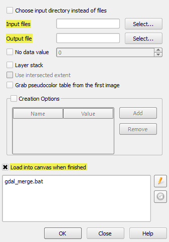 2. In the field Input files, click Select, browse for the tiles to merge, select them and click Open (use the shift key in order to select all). 3. In the field Output files, click Select, set the name of the output mosaic / DSM and select the format GeoTIFF (*…). Choose where to export the new merged file and click Save. 4. (DSM only) check the box No data value and set it to -10000.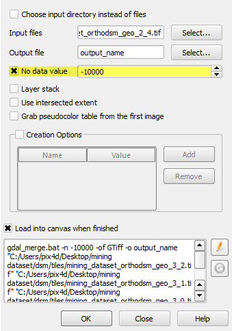5. Check the box Load into canvas when finished in order to see the merged file once it is generated. 6. Click OK.

Previous Versions

QGIS 2: Importing OSM vector layers

QGIS 2.0 integrates OpenStreetMap import as a core functionality.
To get OSM data, use the «Vector → Openstreetmap» menu:

«Load data» will connect to the OSM server and download data. You can skip this step if you already have a .osm XML file.
«Import topology from an XML file» below will convert your .osm file into a spatialite database, and create a db connection.
«Export topology to Spatialite» then allows you to open the database connection, select the type of data you want (points, lines, and polygons) and choose tags to import. Do this three times (clicking ‘Load from DB’ for each) to create three spatialite geometry layers.
Add this layer to your project via the «add a spatialite layer» menu.

OpenStreetMap Plugin (obsolete)

For QGIS older than version 2: The QGIS OSM Plugin lets you load in vector data from OpenStreetMap, and even edit and upload your changes. However, due to a bug related to 64-bit Identifiers, newer data is not read. See the QGIS OSM Plugin page for more info and workarounds.

Shapefiles, PostGIS and other conversion options

There are many ways converting OSM data to other formats which can then be opened within QGIS. In particular note the various options for Shapefiles and PostGIS databases.

Using raster maps from OpenStreetMap

There’s a couple of different approaches to bring in tiles from OpenStreetMap (or from other OpenStreetMap tile providers) :

Install QuickMapServices plugin, find its button on the toolbar and click it to see a list of layers, including OSM layers.

The QGIS OpenLayers Plugin offers another easy way. In QGIS2.0 go to «Plugins» menu -> «Manage Installed Plugins…», then search for OpenLayers under ‘Get More’. In older 1.x QGIS you need to enable the «Plugin Installer» from the Plugin Manager and then from «Plugins» -> «Fetch Python Plugins» and select the «Openlayers Plugin». The list of available OSM tile layers then appears from the «Plugins» -> «OpenLayers plugin» menu. (Note that this process alters the CRS (coordinate reference system) for the QGIS project, and that you may encounter issues with printing the map).

GDAL support is built in, so you can make a GDAL XML config and load this as a raster layer.

The Bigmap service makes it relatively easy to import a georeferenced image created from glued-together map tiles (for a very limited area).

To make OSM layer look smooth make sure you use ESPG:3857 projection and set a scale to start from 1:2257.

You can also import this file to set the scale pyramid for your project:

<qgsScales version="1.0">
<scale value="1:591659030"/>
<scale value="1:295829515"/>
<scale value="1:147914757"/>
<scale value="1:73957378"/>
<scale value="1:36978689"/>
<scale value="1:18489344"/>
<scale value="1:9244672"/>
<scale value="1:4622336"/>
<scale value="1:2311168"/>
<scale value="1:1155584"/>
<scale value="1:577792"/>
<scale value="1:288896"/>
<scale value="1:144448"/>
<scale value="1:72224"/>
<scale value="1:36112"/>
<scale value="1:18056"/>
<scale value="1:9028"/>
<scale value="1:4514"/>
<scale value="1:2257"/>
</qgsScales>

[править] Получение

Геосэмпл можно загрузить целиком, для конкретного ПО или послойно, его также можно посмотреть в работе картсервера или PostGIS.

Внимание: проекты будут полностью функциональны только в случае загрузки комплекта целиком или набора целиком для конкретного ПО.

Название	Название файла	Размер, Mb	Ссылка
Набор целиком	geosample	41.8

Набор целиком по ПО (включает данные, проектные файлы, файлы легенд, если они есть). Ссылка на имени ГИС ведет на официальную страницу. Ссылка на названии файла — на снимок экрана этой ГИС:

Название файла	Версия ПО	Размер, Mb
	9.2	6.7
	3.2	6.8
	6.3	20.4
geosample-geoserver	1.7.6	6.7
	1.1.2	6.7
	7.5	6.3
	4.7	7.4
	1.3	6.7
	2.8	1.5
	1.5
	1.4	6.8
	2.0.3	15.2
	2.3	6.5
	1.0	3.6
	1.1.1	6.8

Данные послойно (в различных форматах):

Название	Название файла	Размер, Mb
Административные границы	admin	0.1
Населенные пункты	settlements	0.1
Гидросеть линейная	hydro-l	0.5
Гидросеть полигональная	hydro-a	0.3
Объекты (POI)	poi-osm	0.2
Дорожная сеть	road-l-osm	1.4
Железные дороги	railroad-l	0.1
Охраняемые природные территории	oopt	0.1
Растительность	veg	1.0
Почвы	soil	0.2
Экорегионы	ecoregions	0.1
Рельеф	relief	7.6
MODIS	modis	8.5

Легенда¶

Область легенды содержит список всех слоёв проекта. Флажок у каждого элемента легенды используется для показа или сокрытия слоя.

Выделенный слой можно перетаскивать выше или ниже других слоёв, меняя их порядок расположения. Порядок расположения слоев означает, что слои находящиеся ближе к верхней части легенды, отрисовываются в окне карты над слоями, перечисленными в легенде ниже.

Примечание

Такое поведение можно переопределить при помощи панели Порядок отрисовки.

Слои можно объединять в группы. Это можно сделать следующими способами:

Поместите курсор мыши в окне легенды карты, щёлкните правой кнопкой мыши и выберите пункт Добавить группу. Введите название группы и нажмите Enter. Теперь можно выделить слой и перетащить его на значок группы.
Выберите несколько слоёв, вызовите контекстное меню и выберите Сгруппировать выделенное. Выделенные ранее слои буду автоматически помещены в новую группу.

Исключить слой из группы можно перетащив его из группы на свободное место в области легенды, или выбрав пункт Сделать элементом первого уровня в контекстном меню слоя. Группы могут быть вложенными.

Флажок возле имени группы даёт возможность переключать видимость всех слоев в группе одним действием.

Содержание контекстного меню, доступного при нажатии правой кнопки мыши на слое, зависит от того, на каком слое в окне легенды вы нажали правой кнопкой — растровом или векторном. Для векторных слоев GRASS Режим редактирования недоступен. Редактирование векторных слоев GRASS рассматривается в разделе .

Контекстное меню для растровых слоев

Увеличить до границ слоя
Увеличить до наилучшего масштаба (100%)
Растянуть значения по текущему охвату
Показать в обзоре
Удалить
Дублировать
Изменить систему координат
Выбрать систему координат слоя для проекта
Сохранить как…
Свойства
Переименовать
Копировать стиль
Добавить группу
Развернуть все
Свернуть все
Обновлять порядок отрисовки

Дополнительно, в зависимости от положения слоя

Сделать элементом первого уровня
Сгруппировать выделенное

Контекстное меню для векторных слоев

Увеличить до границ слоя
Показать в обзоре
Удалить
Дублировать
Изменить систему координат
Выбрать систему координат слоя для проекта
Открыть таблицу атрибутов
Режим редактирования (недоступен для слоёв GRASS)
Сохроанить как…
Сохранить выделение как…
Фильтр…
Показать количество объектов
Свойства
Переименовать
Копировать стиль
Добавить группу
Развернуть все
Свернуть все
Обновлять порядок отрисовки

Дополнительно, в зависимости от положения слоя

Сделать элементом первого уровня
Сгруппировать выделенное

Контекстное меню для групп слоев

Увеличить до группы
Удалить
Изменить систему координат группы
Переименовать
Добавить группу
Развернуть все
Свернуть все
Обновлять порядок отрисовки

При зажатой клавише CTRL можно выделять несколько слоёв или групп одновременно. Это позволит переместить все выделенные слои из одной группы в другую.

Кроме того, можно удалить сразу несколько слоёв или групп, выделив их с зажатой клавишей Ctrl, а затем нажав Ctrl+D. Так можно удалить все выделенные слои или группы из списка слоёв.

Panels and Toolbars¶

From the View menu (or Settings), you can
switch on and off QGIS widgets (Panels ‣) or toolbars
(Toolbars ‣). You can (de)activate any of them by
right-clicking the menu bar or a toolbar and choose the item you want.
Each panel or toolbar can be moved and placed wherever you feel comfortable
within QGIS interface.
The list can also be extended with the activation of .

The toolbar provides access to most of the same functions as the menus, plus
additional tools for interacting with the map. Each toolbar item has pop-up help
available. Hold your mouse over the item and a short description of the tool’s
purpose will be displayed.

Every toolbar can be moved around according to your needs. Additionally,
they can be switched off using the right mouse button context menu, or by
holding the mouse over the toolbars.

The Toolbars menu

Совет

Восстановление панелей инструментов

If you have accidentally hidden a toolbar, you can get it
back by choosing menu option View ‣ Toolbars ‣
(or Settings ‣ Toolbars ‣).
If for some reason a toolbar (or any other widget) totally disappears
from the interface, you’ll find tips to get it back at .

Processing¶

This additional option enriches the Package Layers algorithm and will copy the source layer metadata into the geopackage, so that it will be used as the default metadata for the layer.

This feature was developed by Nyall Dawson

This algorithm retrieves basic raster layer properties such as the size in pixels, pixel dimensions (map units per pixel), number of bands, and no data value.

It is intended for use as a means of extracting these useful properties to use as the input values to other algorithms in a model, such as passing an existing raster’s pixel sizes over to a GDAL raster algorithm.

This feature was developed by Nyall Dawson

The rasterize (vector to raster) GDAL process now supports 3D data, in that it now includes the possibility to use the Z value (elevation) of a feature to extract burn values.

The use of this option indicates that a burn value should be extracted from the “Z” values of the feature. Works with points and lines (linear interpolation along each segment). For polygons, it only works properly if the features are flat (i.e. contain the same Z value for all vertices)

This feature was developed by talledodiego

The Package Layers Algorithm was modified to support saving only selected features

This feature was developed by Stefan Conrads

A new log level property has been added to QgsProcessingContext

This allows algorithms to tune their output based on the logging level.

The qgis_process command line operation has been granted a –verbose switch to enable verbose log output.

This feature was funded by Natural resources Canada Contract: 3000720411

This feature was developed by Nyall Dawson

This development cycle saw a rework of the inner workings of QGIS“ geometry snapper algorithm, which has led to a significant speed boost. Datasets which could take over 10 minutes to process now take less than 10 seconds.

This feature was funded by SwissTierras Colombia

This feature was developed by Mathieu Pellerin